Applied Research In Economics Based On The Solou Model

Abstract

Digitalization of various aspects of socio-economic activity is an urgent direction of the XXI century. The digital economy uses information and communication technologies and keeps the direction of increasing the efficiency and growth rates of the economy. Modern methods for calculating economic efficiency in the process of digitalization of production are based on classical economic and mathematical models. The tasks that need to be solved in the process of empirical research of economic processes and phenomena are associated with the need to ensure the security of the national economy. To analyze, predict the development of economic processes in the field of security of the national economy, economic and mathematical methods and models are used. In this paper, the Solow model is considered and analyzed. The fulcrum of the Solow model is the property of self-replication. This property is expressed with the help of an internal feedback mechanism, according to which part of the production output is returned to the production system in the form of an increase in fixed assets. In the considered Solow model, it is shown that the growth rates of capital investments, fixed assets, consumption fund and other indicators of economic development depend on the choice of the capital investment rate. Since the rate of investment can be controlled, the question of the optimal choice of this parameter is of great practical importance in empirical studies of economic processes and phenomena.

Keywords: Economic and mathematical modeling, Solow model

Introduction

At present, it is difficult to imagine an economy without mathematical models and research methods. The entire economy is mathematized and widely uses mathematical modelling to study economic processes and phenomena.

The modelling method is based on the principle of analogy, i.e. the possibility of studying a real object not directly, but through consideration of a similar and more accessible object, its model (Artamonov et al., 2017; Batkovskiy et al., 2017; Batkovskiy et al., 2015a; Batkovsky & Trofimets 2015; Herchencron, 1962; Kolemaev, 2005; Motorygin et al., 2016; Trofimets, 2009; Solow, 1956, 1957, 1958; Swan, 1956).

Problem Statement

Applied research in economics is, firstly, the analysis of economic objects and processes; secondly, economic forecasting, foreseeing the development of economic processes; thirdly, the development of management decisions. One of the key components of applied research in human-machine systems for planning and managing economic systems is economic and mathematical modelling.

The process of economic and mathematical modelling is usually implemented in four sequential stages:

• statement of the problem and construction of a model (algorithm);
• implementation of the model (modelling algorithm) on a personal computer (PC);
• analysis of the results obtained and transferring them to the original;
• checking the adequacy of the results obtained.

There are four aspects of the application of mathematical methods in solving practical problems in economics:

• improving the system of economic information;
• intensification and improvement of the accuracy of economic calculations;
• deepening the quantitative analysis of economic problems;
• solution of fundamentally new economic problems.

Research Questions

The scope of practical application of the modeling method is limited by the possibilities and effectiveness of formalizing economic problems and situations, as well as the state of information, mathematical, and technical support of the models used (Artamonov et al., 2017; Batkovskiy et al., 2017; Batkovskiy et al., 2015a; Batkovsky & Trofimets, 2015; Motorygin et al., 2016).

The construction of a visual model of economic processes and phenomena in this article is considered on the example of a one-sector macroeconomic model (Batkovsky & Trofimets, 2015; Herchencron, 1962; Kolemaev, 2005; Motorygin et al., 2016; Solow, 1956, 1957, 1958; Swan, 1956; Trofimets, 2009).

Purpose of the Study

At the heart of the one-sector macromodel, which is known in the economic literature as the Solow model, the dynamics of national income is clearly determined by the block diagram shown in Figure 1.

See Full Size >

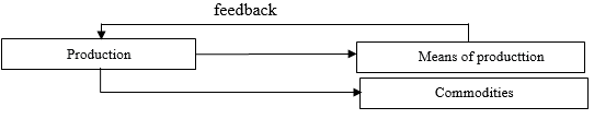
The Solow model reflects the main property of the economy as a dynamic system - its self-reproduction. This property is expressed using an internal feedback mechanism, according to which part of the production output is returned to the production system in the form of an increase in fixed assets.

Let's consider a number of economic concepts (Batkovsky & Trofimets, 2015; Kolemaev, 2005; Solow, 1956, 1957; Trofimets, 2009).

1) The entire production process is described by the Cobb-Douglas aggregated production function:

$Y=Y_0{\left(\frac{K}{K_0}\right)}^a{\left(\frac{L}{L_0}\right)}^{1-a}$ (1)

where Y -; L is the number of employed; K is the volume of fixed assets; a - coefficient of elasticity of labor productivity in terms of capital-labor ratio (0 <a <1). In this case, the index "0" refers to the values of the variables at the initial moment of time t = 0. In economics, expression (1) is called an isoquant or equal output lines.

2) The total product of social production is used for consumption (C) and investment (I):

, (2)

3) Investment (or investment) in the national economy is defined as a part of the national income going to increase fixed assets:

I = sY, (3)

where s is the rate of investment (0 <s <I).

4) The volume of consumption is set by the condition:

C = (1-s) Y, (4)

which follows from relations (2) and (3).

5) The dynamics of fixed assets is determined by the differential equation:

dK / dt = W-mK, (5)

where m is the rate of disposal of fixed assets; W - inputs of new funds; K is the volume of fixed assets. For simplicity, we will assume that the latter are equal to the investment (W = I).

6) The number of employed is determined by the ratio:

$L=L_0{e}^{gt}$ , (6)

where g is the growth rate of the employed (constant); t is time.

Relations (2) - (6) completely set the dynamics of fixed assets. To simplify the subsequentcalculations and analysis of the model, it is convenient to introduce a new variable into consideration:capital-labor ratio:

x =.

Due to the ratio:

x '/ x = K' / K-L '/ L

and representations (1) - (6) we obtain:

$\frac{x^{\text{'}}}{x}=A{\left(\frac{x}{x_0}\right)}^{a-1}-m-g,$ (7)

where

$x_0=\frac{K_0}{L_0},A=s\frac{Y_0}{K_0}$.

As you can see, here it is convenient to switch to dimensionless variables: y '= x' / x,. Equation (7) implies:

$y^{\text{'}}=A{y}^a-By$ (8)

where B = m + g.

So, the study of the one-sector model is reduced to the analysis of the Bernoulli differential equation (8) with the initial condition:

y (0) = 1, (9)

Note that if a = 1 (linear production function), then the solution to equation (8) is the exponential function:

$y=e^{\left(A-B\right)t}$.

Research Methods

Thus, in this case, the capital-labor ratio is either constant (for A = B), or increases (for A> B), or decreases to zero (for A <B).

If a <1, then equation (8) can be solved by the Bernoulli method. To do this, we represent the desired variable as a product of two functions:

y = U V

These functions and because of (8), must satisfy the equation:

$U^{\text{'}}V+U{V}^{\text{'}}=A{\left(UV\right)}^a-BUV$,

from which two conditions follow:

• U'V = -BUV, (10)

$U{V}^{\text{'}}=A{\left(UV\right)}^a$, (11)

From formula (10) we obtain U = exp (-Bt). Substitution of it into (11) leads to the following differential equation for the auxiliary variable

$V^{\text{'}}=A{e}^{\left(\left(1-a\right)Bt\right)V^a}$.

Integration of this equation with the initial condition V (0) = 1, which follows from the initial condition (9), taking into account U (0) = 1, leads to the final solution of the differential equation (8).

This solution looks like this:

$y\left(t\right)={\left(D+\left(1-D\right)e^{\left(-\left(1-a\right)Bt\right)}\right)}^{\frac{1}{1-a}}$ (12)

where $D=\frac{A}{B}=\frac{s{Y}_0}{\left(K_0\left(m+g\right)\right)};$ s is the rate of investment.

Since 0 <a <1, equation (12), when the condition is satisfied, defines an increasing function. Note that with increasing t, the variable y tends to its limiting value:

$y_{00}=D^{\frac{1}{1-a}}$ (13)

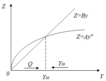
The existence of the limiting value $y_{00}$ is associated with the convexity property of the production function (1) under the condition 0 <a <1. Indeed, from Fig. 2 it follows that in case of $y<y_{00}$ the value of the derivative is positive (since in this case $A{y}^a>By$), as a result of which grows. This fact is indicated in Figure 2 by the arrow Q directed to the right.

If $y>y_{00}$, then the value of the derivative is negative (in this case $A{y}^a<By$), as a result of which the variable decreases. It follows from this that is a stable stationary solution of the differential equation (8).

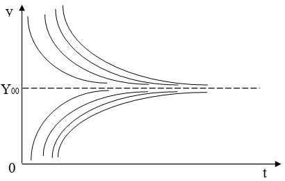
Figure 3 shows the integral curves (12) of the differential equation (8), demonstrating the stability of the solution $y=y_{00}$.

To determine the dependence of fixed assets on time, formula (6) and (12) are used. After identical transformations we get:

$K=K_0\left(\frac{K}{L}\right)\left(\frac{L_0}{K_0}\right)\left(L/L_0\right)=K_{0}y\left(t\right)e^{gt}$ (14)

Findings

As we can see, because of the tendency of y (t) to $y_{00}$ at $t\to \infty$, the growth rates of fixed assets over time practically coincide with the growth rates of the number of employed. Thanks to (3) and (4), consumption C and investment I also increase at sufficiently high values of t, and their growth rates practically coincide with the growth rate of the employed. This situation is called balanced growth

See Full Size >

See Full Size >

Conclusion

So, for model (1) - (5) at a constant rate of capital investment, the balanced growth mode has the property that all the trajectories of the model converge to it.

Note that with an increase in the rate of capital investment, the value increases, and with an increase in the rate of population growth, decreases. This follows from the equality:

$D=\frac{s{Y}_0}{\left(K_0\left(m+g\right)\right)}$.

Therefore, regardless of the initial data, all solutions of the one-sector model equation converge to an equilibrium trajectory $y=y_{00}$. In this case, the value $y_{00}$ depends on the rate of investment

The latter means that in the model under consideration, the capital investment rate is an essential factor, on the choice of which the growth rates of capital investments, fixed assets, consumption fund and other indicators of economic development depend.

Since the rate of investment can be controlled, the question of the optimal choice of this parameter is of great practical importance in empirical studies of economic processes and phenomena.

References

• Artamonov, V. S., Ivanov, A. Y., Sharapov, S. V., Trofimets, E. N., & Trofimets, V. Ya. (2017). Information systems and processes in the analytical training of management scholars. Espacios, 38(25), 18.

• Batkovskiy, A. M., Semenova, E. G., Trofimets, E. N., Trofimets, V. Y., & Fomina, A. V. (2017). Statistical simulation of the break-even point in the margin analysis of the company. Journal of Applied Economic Sciences. Romania: European Research Centre of Managerial Studies in Business Administration, XII, 2(48), 558-570.

• Batkovskiy, A. M., Semenova, E. G., Trofimets, V. Ya., Trofimets, E. N., & Fomina, A. V. (2015a). Automated Rating of Financial and Economic Condition of Companies. Mediterranean Journal of Social Sciences. MCSER Publishing, 6(5), 4, 297-308.

• Batkovsky, A. M., & Trofimets, V. Ya. (2015). Decision Support Systems with Modules of Applied Mathematical Models and Methods. Problems of Radioelectronics, 9, 253-275.

• Herchencron, A. (1962). The Approach to European Industrialization: A Postscript. Economic Backwardness in Historical Perspective: A Book of Essays. Cambridge (Mass.).

• Kolemaev, V. A. (2005). Economic and mathematical modeling. Modeling of macroeconomic processes and systems. UNITI-DANA.

• Motorygin, Y. D., Artamonov, V. S., Maximov, A. V., Trofimets, V. Ya., & Trofimets, E. N. (2016). Management of the Formation of Rating Preferences of Economic Entities upon Collective Choice. International Journal of Economics and Financial Issues, 6(4), 1956-1964.

• Solow, R. M. (1956). A Contribution to the Theory of Economic Growth. The Quarterly Journal of Economics, 70(1).

• Solow, R. M. (1957). Technical Change and the Aggregate Production Function. The Review of Economics and Statistics, 39(3).

• Solow, R. M. (1958). A Skeptical Note on the Constancy of Relative Shares. American Economic Review, 48(4).

• Swan, T. W. (1956). Economic growth and capital accumulation. Economic Record, 32(2).

• Trofimets, E. N. (2009). Conceptual model of the scientific and methodological apparatus for solving professionally oriented economic problems. Bulletin of the Peoples' Friendship University of Russia. Series "Informatization of Education", 4, 107-117.